


Oberschwingungen in Mehrphasenstromsystemen
Im Kapitel über Mischfrequenzsignale haben wir das Konzept der Oberschwingungen untersucht in Wechselstromsystemen:Frequenzen, die ganzzahlige Vielfache der Grundfrequenz der Quelle sind.
Bei Wechselstromnetzen, bei denen die von einem Wechselstromgenerator (Wechselstromgenerator) kommende Wellenform der Quellenspannung eine unverzerrte Sinuswelle mit einer einzigen Frequenz sein soll, sollte kein Oberwellengehalt vorhanden sein . . . idealerweise.
Nichtlineare Komponenten in Wechselstromsystemen
Dies wäre wahr, wenn es nicht nichtlineare Komponenten gäbe . Nichtlineare Komponenten ziehen Strom überproportional zur Quellenspannung und verursachen nicht-sinusförmige Stromwellenformen.
Beispiele für nichtlineare Komponenten sind Gasentladungslampen, Halbleiter-Leistungssteuergeräte (Dioden, Transistoren, SCRs, TRIACs), Transformatoren (der Magnetisierungsstrom der Primärwicklung ist aufgrund der B/H-Sättigungskurve des Kerns normalerweise nicht sinusförmig) und Elektromotoren (wiederum, wenn Magnetfelder im Kern des Motors nahe der Sättigung arbeiten).
Auch Glühlampen erzeugen leicht nicht-sinusförmige Ströme, da sich der Wendelwiderstand durch schnelle Temperaturschwankungen während des Zyklus ändert.
Wie wir im Kapitel über gemischte Frequenzen gelernt haben, ist jede Die Verzerrung einer ansonsten sinusförmigen Wellenform stellt das Vorhandensein von harmonischen Frequenzen dar.
Wenn die fragliche nicht-sinusförmige Wellenform oberhalb und unterhalb ihrer durchschnittlichen Mittellinie symmetrisch ist, sind die harmonischen Frequenzen nur ungerade ganzzahlige Vielfache der Grundfrequenz der Quelle, ohne gerade ganzzahlige Vielfache.
Die meisten nichtlinearen Lasten erzeugen Stromwellenformen wie diese, sodass geradzahlige Harmonische (2., 4., 6., 8., 10., 12. usw.) in den meisten Wechselstromnetzen nicht oder nur minimal vorhanden sind.
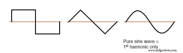
Beispiele für symmetrische Wellenformen – nur ungerade Harmonische.
Beispiele für unsymmetrische Wellenformen mit geraden Oberwellen sind in der Abbildung unten als Referenz gezeigt.
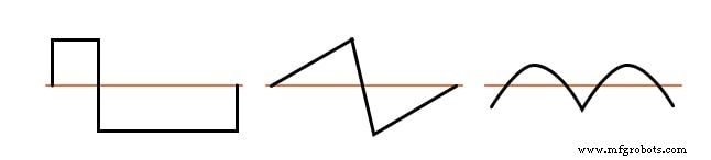
Beispiele für unsymmetrische Wellenformen – gerade Harmonische vorhanden.
Auch wenn die Hälfte der möglichen harmonischen Frequenzen durch die typischerweise symmetrische Verzerrung nichtlinearer Lasten eliminiert wird, können die ungeraden Harmonischen dennoch Probleme verursachen. Einige dieser Probleme gelten allgemein für alle Stromversorgungssysteme, einphasig oder nicht.
Eine Überhitzung des Transformators durch Wirbelstromverluste kann beispielsweise in jedem auftreten Wechselstromnetz mit erheblichem Oberwellengehalt.
Es gibt jedoch einige Probleme, die durch Oberwellenströme verursacht werden, die spezifisch für mehrphasige Stromversorgungssysteme sind, und diesen Problemen ist dieser Abschnitt speziell gewidmet.
SPICE-Simulation bezüglich harmonischer Effekte
Es ist hilfreich, nichtlineare Lasten in SPICE simulieren zu können, um viel komplexe Mathematik zu vermeiden und ein intuitiveres Verständnis von harmonischen Effekten zu erhalten.
Lineare AC-Systemsimulation
Zuerst beginnen wir unsere Simulation mit einem sehr einfachen Wechselstromkreis:einer einzelnen Sinusspannungsquelle mit einer rein linearen Last und allen zugehörigen Widerständen:
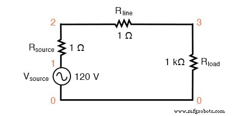
SPICE-Schaltung mit einer einzelnen Sinuswellenquelle.
Die RQuelle und RLinie Widerstände in dieser Schaltung imitieren nicht nur die reale Welt:Sie bieten auch praktische Shunt-Widerstände zum Messen von Strömen in der SPICE-Simulation:Durch das Ablesen der Spannung an einem 1--Widerstand erhalten Sie eine direkte Anzeige des Stroms durch ihn, da E =IR .
Eine SPICE-Simulation dieser Schaltung (SPICE-Listing:„lineare Lastsimulation“) mit Fourier-Analyse der über RLeitung gemessenen Spannung sollte uns den Oberwellengehalt des Netzstroms dieser Schaltung zeigen. Da wir von Natur aus vollständig linear sind, sollten wir außer der 1. (Grundschwingung) von 60 Hz keine anderen Oberwellen erwarten, wenn eine 60-Hz-Quelle angenommen wird.
Siehe SPICE-Ausgabe „Fourier-Komponenten des Einschwingverhaltens v(2,3)“ und die Abbildung unten.
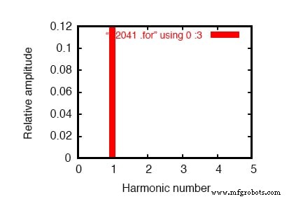
Frequenzbereichsdiagramm einer einzelnen Frequenzkomponente. Siehe SPICE-Listing:„lineare Lastsimulation“.
Ein .plot-Befehl erscheint in der SPICE-Netzliste, und normalerweise würde dies zu einer Sinuskurven-Grafikausgabe führen. In diesem Fall habe ich jedoch der Kürze halber die Wellenformanzeige absichtlich weggelassen – der Befehl .plot befindet sich in der Netzliste, nur um eine Eigenart der Fourier-Transformationsfunktion von SPICE zu erfüllen.
Keine diskrete Fourier-Transformation ist perfekt, und daher sehen wir sehr kleine harmonische Ströme (im Pico-Ampere-Bereich!) für alle Frequenzen bis zur 9. .
Wir zeigen 0,1198 Ampere (1,198E-01) für die „Fourier-Komponente“ der 1. Harmonischen oder die Grundfrequenz, die unser erwarteter Laststrom ist:ca. 120 mA bei einer Quellenspannung von 120 Volt und einem Lastwiderstand von 1 kΩ.
Einfache nichtlineare einphasige AC-Systemsimulation
Als nächstes möchte ich eine nichtlineare Last simulieren, um harmonische Ströme zu erzeugen. Dies kann auf zwei grundsätzlich unterschiedliche Arten erfolgen. Eine Möglichkeit besteht darin, eine Last mit nichtlinearen Komponenten wie Dioden oder anderen Halbleiterbauelementen zu entwerfen, die mit SPICE einfach simuliert werden können. Eine andere besteht darin, einige Wechselstromquellen parallel zum Lastwiderstand hinzuzufügen.
Letztere Methode wird häufig von Ingenieuren zur Simulation von Oberwellen bevorzugt, da sich Stromquellen mit bekanntem Wert besser für die mathematische Netzwerkanalyse eignen als Komponenten mit hochkomplexen Ansprecheigenschaften.
Da wir SPICE die ganze mathematische Arbeit überlassen würden, würde uns die Komplexität einer Halbleiterkomponente keine Probleme bereiten, aber da Stromquellen fein abgestimmt werden können, um jede beliebige Strommenge zu erzeugen (eine praktische Funktion), werde ich Wählen Sie den letztgenannten Ansatz, der in der folgenden Abbildung und im SPICE-Listing „Nichtlineare Lastsimulation“ gezeigt wird.
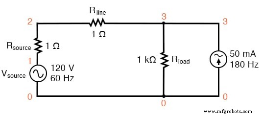
SPICE-Schaltung:60-Hz-Quelle mit hinzugefügter 3. Harmonischer.
In dieser Schaltung haben wir eine Stromquelle mit einer Größe von 50 mA und einer Frequenz von 180 Hz, was dem Dreifachen der Quellenfrequenz von 60 Hz entspricht. Parallel zum 1-kΩ-Lastwiderstand geschaltet, addiert sich sein Strom mit dem des Widerstands zu einem nicht-sinusförmigen Gesamtleitungsstrom.
Ich zeige das Wellenformdiagramm in der Abbildung unten, nur damit Sie die Auswirkungen dieses Stroms der 3. Harmonischen auf den Gesamtstrom sehen können, der normalerweise eine einfache Sinuswelle wäre.
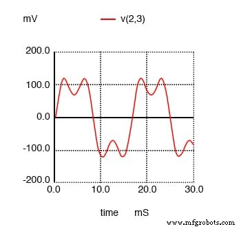
SPICE-Zeitbereichsdiagramm, das die Summe der 60-Hz-Quelle und der dritten Harmonischen von 180 Hz zeigt.
Fourier-Komponenten der Übergangsantwort v(2,3) Gleichstromkomponente =1,349E-11 harmonische Frequenz Fourier normiert phasennormiert keine (hz) Komponente Komponente (Grad) Phase (Grad) 1 6.000E+01 1.198E-01 1.000000 -72.000 0.000 2 1.200E+02 1.609E-11 0.000000 67.570 139.570 3 1.800E+02 4.990E-02 0.416667 144.000 216.000 4 2.400E+02 1.074E-10 0.000000 -169.546 -97.546 5 3.000E+02 3.871E-11 0.000000 169.582 241.582 6 3.600E+02 5.736E-11 0.000000 140.845 212.845 7 4.200E+02 8.407E-11 0.000000 177.071 249.071 8 4.800E+02 1.329E-10 0.000000 156.772 228.772 9 5.400E+02 2.619E-10 0.000000 160.498 232.498 Gesamtklirrfaktor =41,6666663 Prozent
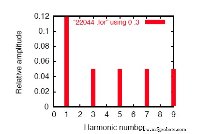
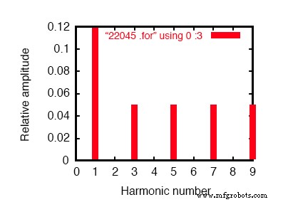
SPICE-Fourier-Plot mit einer 60-Hz-Quelle und einer dritten Harmonischen von 180 Hz.
Bei der Fourier-Analyse (siehe Abbildung oben und „Fourier-Komponenten der Einschwingantwort v(2,3)“) werden die gemischten Frequenzen entmischt und separat dargestellt.
Hier sehen wir die gleichen 0,1198 Ampere 60 Hz (Grund-) Strom wie in der ersten Simulation, aber in der 3. harmonischen Reihe sehen wir 49,9 mA:unsere 50 mA, 180 Hz Stromquelle bei der Arbeit. Warum sehen wir nicht die gesamten 50 mA durch die Leitung?
Da diese Stromquelle über den 1-kΩ-Lastwiderstand angeschlossen ist, wird ein Teil ihrer Ströme durch die Last geleitet und fließt nie durch die Leitung zurück zur Quelle. Dies ist eine unvermeidliche Folge dieser Art von Simulation, bei der ein Teil der Last „normal“ ist (ein Widerstand) und der andere Teil von einer Stromquelle imitiert wird.
Nichtlineare einphasige AC-Systemsimulation mit mehreren Stromquellen
Wenn wir der „Last“ weitere Stromquellen hinzufügen würden, würden wir eine weitere Verzerrung der Linienstromwellenform von der idealen Sinuswellenform sehen, und jeder dieser harmonischen Ströme würde in der Aufschlüsselung der Fourier-Analyse erscheinen. Siehe folgende Abbildung und das SPICE-Listing:„Nichtlineare Lastsimulation“.
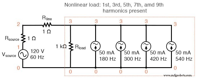
Nichtlineare Last:1., 3., 5., 7. und 9. Harmonische vorhanden.
Nichtlineare Lastsimulation vsource 1 0 sin(0 120 60 0 0) Quelle 1 2 1 rline 2 3 1 rload 3 0 1k i3har 3 0 sin(0 50m 180 0 0) i5har 3 0 sin(0 50m 300 0 0) i7har 3 0 sin(0 50m 420 0 0) i9har 3 0 sin(0 50m 540 0 0) .Optionen itl5=0 .tran 0.5m 30m 0 1u .plot tran v(2,3) .vier 60 v(2,3) .end
Fourier-Komponenten der Übergangsantwort v(2,3) Gleichstromkomponente =6,299E-11 harmonische Frequenz Fourier normiert phasennormiert keine (hz) Komponente Komponente (Grad) Phase (Grad) 1 6.000E+01 1.198E-01 1.000000 -72.000 0.000 2 1.200E+02 1.900E-09 0.000000 -93.908 -21.908 3 1.800E+02 4.990E-02 0.416667 144.000 216.000 4 2.400E+02 5.469E-09 0.000000 -116.873 -44.873 5 3.000E+02 4.990E-02 0.416667 0.000 72.000 6 3.600E+02 6.271E-09 0.000000 85.062 157.062 7 4.200E+02 4.990E-02 0.416666 -144.000 -72.000 8 4.800E+02 2.742E-09 0.000000 -38.781 33.219 9 5.400E+02 4.990E-02 0.416666 72.000 144.000 Gesamtklirrfaktor =83,333296 Prozent
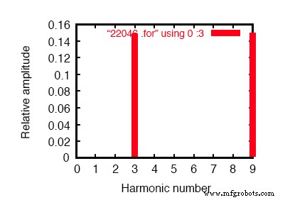
Fourier-Analyse:"Fourier-Komponenten der Übergangsantwort v(2,3)".
Wie Sie der Fourier-Analyse (Abbildung oben) entnehmen können, ist jede harmonische Stromquelle mit jeweils 49,9 mA gleichermaßen im Netzstrom vertreten. Bisher ist dies nur eine einphasige Stromsystemsimulation.
Dreiphasen-AC-Systemsimulation
Interessanter wird es, wenn wir es zu einer dreiphasigen Simulation machen. Es werden zwei Fourier-Analysen durchgeführt:eine für die Spannung über einem Leitungswiderstand und eine für die Spannung über dem Neutralwiderstand.
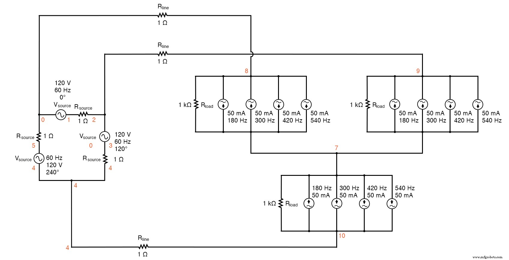
Wie zuvor gibt das Ablesen von Spannungen an festen Widerständen von jeweils 1 direkte Hinweise auf den Strom durch diese Widerstände. Siehe die Abbildung unten und die SPICE-Liste „Y-Y Quelle/Last 4-Leiter-System mit Oberwellen“.
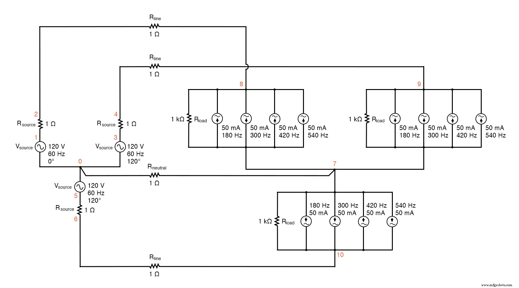
SPICE-Schaltung:Analyse von „Netzstrom“ und „Neutralstrom“, Y-Y Quelle/Last 4-Leiter-System mit Oberwellen.
Y-Y Quelle/Last 4-Leiter-System mit Oberwellen * * Phase1 Spannungsquelle und r (120 V /_ 0 Grad) vsource1 1 0 sin(0 120 60 0 0) Quelle1 1 2 1 * * Phase2 Spannungsquelle und r (120 V /_ 120 Grad) vsource2 3 0 sin(0 120 60 5.55555m 0) Quelle2 3 4 1 * * Phase3 Spannungsquelle und r (120 V /_ 240 Grad) vsource3 5 0 sin(0 120 60 11.1111m 0) rsource3 5 6 1 * * Leitungs- und Neutralleiterwiderstände rline1 2 8 1 rline2 4 9 1 rline3 6 10 1 rneutral 0 7 1 * * Phase 1 der Last rload1 8 7 1k i3har1 8 7 sin(0 50m 180 0 0) i5har1 8 7 sin(0 50m 300 0 0) i7har1 8 7 sin(0 50m 420 0 0) i9har1 8 7 sin(0 50m 540 0 0) * * Phase 2 der Last rload2 9 7 1k i3har2 9 7 sin(0 50m 180 5.55555m 0) i5har2 9 7 sin(0 50m 300 5.55555m 0) i7har2 9 7 sin(0 50m 420 5.55555m 0) i9har2 9 7 sin(0 50m 540 5.55555m 0) * * Phase 3 der Last rload3 10 7 1k i3har3 10 7 sin(0 50m 180 11,1111m 0) i5har3 10 7 sin(0 50m 300 11,1111m 0) i7har3 10 7 sin(0 50m 420 11,1111m 0) i9har3 10 7 sin(0 50m 540 11,1111m 0) * * Analysekram .Optionen itl5=0 .tran 0.5m 100m 12m 1u .plot tran v(2,8) .vier 60 v(2,8) .plot tran v(0,7) .vier 60 v(0,7) .Ende
Fourier-Analyse des Leitungsstroms:
Fourier-Komponenten der Übergangsantwort v(2,8) Gleichstromkomponente =-6.404E-12 harmonische Frequenz Fourier normiert phasennormiert keine (hz) Komponente Komponente (Grad) Phase (Grad) 1 6.000E+01 1.198E-01 1.000000 0.000 0.000 2 1,200E+02 2,218E-10 0,000000 172,985 172,985 3 1.800E+02 4.975E-02 0.415423 0.000 0.000 4 2,400E+02 4,236E-10 0,000000 166,990 166,990 5 3.000E+02 4.990E-02 0.416667 0.000 0.000 6 3.600E+02 1.877E-10 0.000000 -147.146 -147.146 7 4.200E+02 4.990E-02 0.416666 0.000 0.000 8 4.800E+02 2.784E-10 0.000000 -148.811 -148.811 9 5.400E+02 4.975E-02 0.415422 0.000 0.000 Gesamtklirrfaktor =83,209009 Prozent
Fourier-Analyse des Netzstroms in einem symmetrischen Y-Y-System.
Fourier-Analyse des Neutralstroms:
Fourier-Komponenten der Übergangsantwort v(0,7) Gleichstromkomponente =1,819E-10 harmonische Frequenz Fourier normiert phasennormiert keine (hz) Komponente Komponente (Grad) Phase (Grad) 1 6.000E+01 4.337E-07 1.000000 60.018 0.000 2 1,200E+02 1,869E-10 0,000431 91,206 31,188 3 1.800E+02 1.493E-01 344147.7638 -180.000 -240.018 4 2.400E+02 1.257E-09 0.002898 -21.103 -81.121 5 3.000E+02 9.023E-07 2.080596 119.981 59.963 6 3,600E+02 3,396E-10 0,000783 15,882 -44,136 7 4,200E+02 1,264E-06 2,913955 59,993 -0,025 8 4.800E+02 5.975E-10 0.001378 35.584 -24.434 9 5.400E+02 1.493E-01 344147.4889 -179.999 -240.017
Die Fourier-Analyse des Nullleiterstroms zeigt andere als keine Oberwellen! Vergleichen Sie mit dem Leitungsstrom in der Abbildung oben.
Dies ist ein symmetrisches Y-Y-Stromsystem, bei dem jede Phase mit dem zuvor simulierten einphasigen Wechselstromsystem identisch ist. Folglich überrascht es nicht, dass die Fourier-Analyse für den Netzstrom in einer Phase des 3-Phasen-Systems nahezu identisch mit der Fourier-Analyse für den Netzstrom im Einphasen-System ist:ein Grundschwingungs-(60 Hz)-Netzstrom von 0,1198 Ampere und ungeradzahlige harmonische Ströme von jeweils ca. 50 mA.
Siehe die Abbildung oben und die Fourier-Analyse:„Fourier-Komponenten der transienten Antwort v(2,8)“
Überraschend ist hier die Analyse für den Neutralleiterstrom, bestimmt durch den Spannungsabfall am RNeutral Widerstand zwischen SPICE-Knoten 0 und 7.
Bei einer symmetrischen 3-Phasen-Y-Last würden wir erwarten, dass der Neutralstrom null ist. Jeder Phasenstrom – der für sich allein durch den Neutralleiter zurück zur speisenden Phase an der Quelle Y fließen würde – sollte sich in Bezug auf den Neutralleiter gegenseitig aufheben, da sie alle die gleiche Größe haben und alle um 120° verschoben sind.
In einem System ohne Oberwellenströme ist dies ist was passiert, so dass kein Strom durch den Neutralleiter fließt.
Auswirkungen von Oberschwingungsströmen im System
Dasselbe können wir jedoch nicht für harmonisch sagen Ströme im gleichen System.
Beachten Sie, dass der Grundfrequenzstrom (60 Hz oder die 1. Harmonische) im Neutralleiter praktisch nicht vorhanden ist. Unsere Fourier-Analyse zeigt nur 0,4337 µA der 1. Harmonischen beim Lesen der Spannung über RNeutral . Das gleiche gilt für die 5. und 7. Harmonische, wobei beide Ströme eine vernachlässigbare Größe haben.
Im Neutralleiter hingegen sind die 3. und 9. Harmonische mit jeweils 149,3 mA (1.493E-01 Volt über 1 ) stark vertreten! Dies sind fast 150 mA oder das Dreifache der Werte der Stromquellen einzeln.
Bei drei Quellen pro harmonischer Frequenz in der Last scheint es, als würden unsere 3. und 9. Harmonischen in jeder Phase addieren um den neutralen Strom zu bilden. Siehe Fourier-Analyse:„Fourier-Komponenten der transienten Antwort v(0,7)“
Zeitbereichsdiagrammanalyse
Genau das passiert, obwohl es vielleicht nicht klar ist, warum das so ist.
Der Schlüssel zum Verständnis wird in einem Zeitbereichsdiagramm der Phasenströme verdeutlicht. Untersuchen Sie dieses Diagramm der symmetrischen Phasenströme über die Zeit mit einer Phasenfolge von 1-2-3. (Abbildung unten)
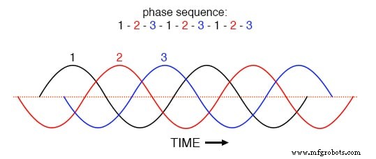
Phasenfolge 1-2-3-1-2-3-1-2-3 von Wellen mit gleichem Abstand.
Wenn die drei Grundwellenformen gleichmäßig über die Zeitachse des Diagramms verschoben sind, ist leicht zu erkennen, wie sie sich gegenseitig aufheben würden, um einen resultierenden Strom von Null im Neutralleiter zu ergeben. Betrachten wir jedoch, wie eine 3. harmonische Wellenform für Phase 1 aussehen würde, wenn sie dem Diagramm in der folgenden Abbildung überlagert ist.
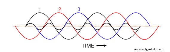
Die dritte harmonische Wellenform für Phase-1 überlagert dreiphasigen Grundwellenformen.
Beobachten Sie, wie diese harmonische Wellenform die gleiche Phasenbeziehung zu der 2. und 3. Grundwellenform hat wie bei der 1.:in jeder positiven Halbwelle von beliebig der Grundwellenformen finden Sie genau zwei positive Halbwellen und eine negative Halbwelle der harmonischen Wellenform.
Das bedeutet, dass die 3. harmonischen Wellenformen von drei 120° phasenverschobenen Grundfrequenzwellenformen tatsächlich in Phase sind miteinander. Die in Drehstromsystemen allgemein angenommene Phasenverschiebungszahl von 120° gilt nur für die Grundfrequenzen, nicht für deren harmonische Vielfache!
Wenn wir alle drei Wellenformen der 3. Harmonischen in demselben Diagramm darstellen würden, würden wir sehen, dass sie sich genau überlappen und als eine einzige, einheitliche Wellenform erscheinen (in Fettdruck in (Abbildung unten) gezeigt.
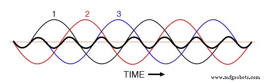
Dritte Harmonische für die Phasen 1, 2, 3 fallen alle zusammen, wenn sie den dreiphasigen Grundwellenformen überlagert werden.
Mathematische Analyse des Zeitbereichsgraphen
Für mathematisch veranlagte Personen kann dieses Prinzip symbolisch ausgedrückt werden. Angenommen, A repräsentiert eine Wellenform und B eine andere, beide auf der gleichen Frequenz, aber um 120° phasenverschoben. Nennen wir die 3. Harmonische jeder Wellenform A’ und B' , bzw.
Die Phasenverschiebung zwischen A’ und B' nicht 120° ist (das ist die Phasenverschiebung zwischen A und B ), aber dreimal so viel, weil das A’ und B' Wellenformen wechseln dreimal so schnell wie A und B . Die Verschiebung zwischen den Wellenformen wird nur in Form des Phasenwinkels . genau ausgedrückt wenn dieselbe Winkelgeschwindigkeit angenommen wird.
Wenn Wellenformen unterschiedlicher Frequenz in Beziehung gesetzt werden, lässt sich die Phasenverschiebung am genauesten in Bezug auf die Zeit darstellen; und die Zeitverschiebung zwischen A’ und B' entspricht 120° bei einer dreimal niedrigeren Frequenz oder 360° bei der Frequenz von A’ und B' . Eine Phasenverschiebung von 360° entspricht einer Phasenverschiebung von 0°, also überhaupt keine Phasenverschiebung.
Also, A’ und B' müssen in Phase miteinander sein:
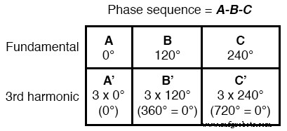
Diese Eigenschaft der 3. Harmonischen in einem Drehstromsystem gilt auch für alle ganzzahligen Vielfachen der 3. Harmonischen.
Somit sind nicht nur die 3. Harmonischen jeder Grundwellenform in Phase miteinander, sondern auch die 6. Harmonische, die 9. Harmonische, die 12. Harmonische, die 15. Harmonische, die 18. Harmonische, die 21. Harmonische und so weiter.
Da nur ungeradzahlige Harmonische in Systemen auftreten, in denen die Wellenformverzerrung symmetrisch um die Mittellinie ist – und die meisten nichtlinearen Lasten symmetrische Verzerrungen erzeugen – sind geradzahlige Vielfache der 3. Harmonischen (6., 12., 18. usw.) im Allgemeinen nicht signifikant, so dass nur die ungeradzahlige Vielfache (3., 9., 15., 21. usw.), um signifikant zu den neutralen Strömen beizutragen.
In mehrphasigen Netzen mit einer anderen Anzahl von Phasen als drei tritt dieser Effekt mit Oberwellen des gleichen Vielfachen auf. Zum Beispiel wären die harmonischen Ströme, die sich im Neutralleiter eines 4-Phasen-Systems mit Sternschaltung hinzufügen, bei dem die Phasenverschiebung zwischen den Grundwellenformen 90° beträgt, der 4., 8., 12., 16., 20. usw. P>
Triple Harmonics
Aufgrund ihrer Fülle und Bedeutung in Drehstromnetzen haben die 3. Harmonische und ihre Vielfachen einen eigenen besonderen Namen:Triple Harmonics .
Alle Triplen-Oberschwingungen addieren sich im Neutralleiter einer 4-adrigen Y-verbundenen Last. In Stromversorgungssystemen mit erheblicher nichtlinearer Belastung können die Ströme der Triplen-Oberschwingung groß genug sein, um eine Überhitzung der Neutralleiter zu verursachen.
Dies ist sehr problematisch, da andere Sicherheitsbedenken einen Überstromschutz von Neutralleitern verbieten und daher keine automatische Unterbrechung dieser hohen Ströme vorgesehen ist.
Analyse der Auswirkungen von Triplen-Oberschwingungen in einer Y-Y-Schaltung
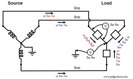
Die folgende Abbildung zeigt, wie sich die an der Last erzeugten dreifachen Oberwellenströme innerhalb des Neutralleiters addieren. Das Symbol „ω“ wird verwendet, um die Winkelgeschwindigkeit darzustellen und ist mathematisch äquivalent zu 2πf. „ω“ steht für die Grundfrequenz, „3ω“ für die 3. Harmonische, „5ω“ für die 5. Harmonische und so weiter:(Abbildung unten)
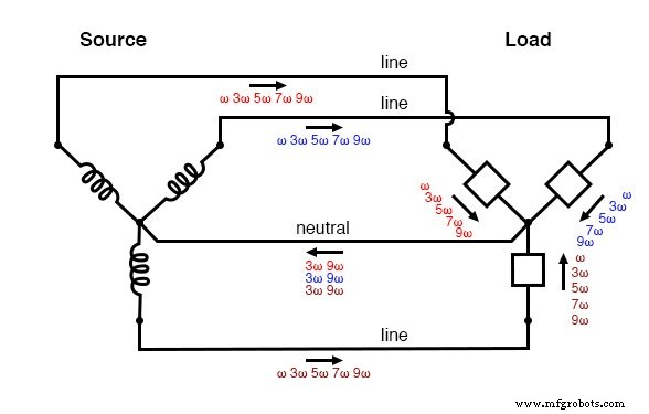
„Y-Y“ Quelle/Last verdreifachen:Oberschwingungsströme addieren sich im Neutralleiter.
Um diese zusätzlichen Tripelströme abzuschwächen, könnte man versucht sein, den Neutralleiter vollständig zu entfernen. If there is no neutral wire in which triplen currents can flow together, then they won’t, right?
Unfortunately, doing so just causes a different problem:the load’s “Y” center-point will no longer be at the same potential as the source’s, meaning that each phase of the load will receive a different voltage than what is produced by the source.
We’ll re-run the last SPICE simulation without the 1 Ω Rneutral resistor and see what happens:
Y-Y source/load (no neutral) with harmonics * * phase1 voltage source and r (120 v / 0 deg) vsource1 1 0 sin(0 120 60 0 0) rsource1 1 2 1 * * phase2 voltage source and r (120 v / 120 deg) vsource2 3 0 sin(0 120 60 5.55555m 0) rsource2 3 4 1 * * phase3 voltage source and r (120 v / 240 deg) vsource3 5 0 sin(0 120 60 11.1111m 0) rsource3 5 6 1 * * line resistances rline1 2 8 1 rline2 4 9 1 rline3 6 10 1 * * phase 1 of load rload1 8 7 1k i3har1 8 7 sin(0 50m 180 0 0) i5har1 8 7 sin(0 50m 300 0 0) i7har1 8 7 sin(0 50m 420 0 0) i9har1 8 7 sin(0 50m 540 0 0) * * phase 2 of load rload2 9 7 1k i3har2 9 7 sin(0 50m 180 5.55555m 0) i5har2 9 7 sin(0 50m 300 5.55555m 0) i7har2 9 7 sin(0 50m 420 5.55555m 0) i9har2 9 7 sin(0 50m 540 5.55555m 0) * * phase 3 of load rload3 10 7 1k i3har3 10 7 sin(0 50m 180 11.1111m 0) i5har3 10 7 sin(0 50m 300 11.1111m 0) i7har3 10 7 sin(0 50m 420 11.1111m 0) i9har3 10 7 sin(0 50m 540 11.1111m 0) * * analysis stuff .options itl5=0 .tran 0.5m 100m 12m 1u .plot tran v(2,8) .four 60 v(2,8) .plot tran v(0,7) .four 60 v(0,7) .plot tran v(8,7) .four 60 v(8,7) .Ende
Fourier analysis of line current:
Fourier components of transient response v(2,8) dc component =5.423E-11 harmonic frequency Fourier normalized phase normalized no (hz) component component (deg) phase (deg) 1 6.000E+01 1.198E-01 1.000000 0.000 0.000 2 1.200E+02 2.388E-10 0.000000 158.016 158.016 3 1.800E+02 3.136E-07 0.000003 -90.009 -90.009 4 2.400E+02 5.963E-11 0.000000 -111.510 -111.510 5 3.000E+02 4.990E-02 0.416665 0.000 0.000 6 3.600E+02 8.606E-11 0.000000 -124.565 -124.565 7 4.200E+02 4.990E-02 0.416668 0.000 0.000 8 4.800E+02 8.126E-11 0.000000 -159.638 -159.638 9 5.400E+02 9.406E-07 0.000008 -90.005 -90.005 total harmonic distortion =58.925539 percent
Fourier analysis of voltage between the two “Y” center-points:
Fourier components of transient response v(0,7) dc component =6.093E-08 harmonic frequency Fourier normalized phase normalized no (hz) component component (deg) phase (deg) 1 6.000E+01 1.453E-04 1.000000 60.018 0.000 2 1.200E+02 6.263E-08 0.000431 91.206 31.188 3 1.800E+02 5.000E+01 344147.7879 -180.000 -240.018 4 2.400E+02 4.210E-07 0.002898 -21.103 -81.121 5 3.000E+02 3.023E-04 2.080596 119.981 59.963 6 3.600E+02 1.138E-07 0.000783 15.882 -44.136 7 4.200E+02 4.234E-04 2.913955 59.993 -0.025 8 4.800E+02 2.001E-07 0.001378 35.584 -24.434 9 5.400E+02 5.000E+01 344147.4728 -179.999 -240.017 total harmonic distortion =************ percent
Fourier analysis of load phase voltage:
Fourier components of transient response v(8,7) dc component =6.070E-08 harmonic frequency Fourier normalized phase normalized no (hz) component component (deg) phase (deg) 1 6.000E+01 1.198E+02 1.000000 0.000 0.000 2 1.200E+02 6.231E-08 0.000000 90.473 90.473 3 1.800E+02 5.000E+01 0.417500 -180.000 -180.000 4 2.400E+02 4.278E-07 0.000000 -19.747 -19.747 5 3.000E+02 9.995E-02 0.000835 179.850 179.850 6 3.600E+02 1.023E-07 0.000000 13.485 13.485 7 4.200E+02 9.959E-02 0.000832 179.790 179.789 8 4.800E+02 1.991E-07 0.000000 35.462 35.462 9 5.400E+02 5.000E+01 0.417499 -179.999 -179.999 total harmonic distortion =59.043467 percent
Strange things are happening, indeed.
First, we see that the triplen harmonic currents (3rd and 9th) all but disappear in the lines connecting a load to source. The 5th and 7th harmonic currents are present at their normal levels (approximately 50 mA), but the 3rd and 9th harmonic currents are of negligible magnitude.
Second, we see that there is a substantial harmonic voltage between the two “Y” center-points, between which the neutral conductor used to connect. According to SPICE, there are 50 volts of both 3rd and 9th harmonic frequency between these two points, which is definitely not normal in a linear (no harmonics), balanced Y system.
Finally, the voltage as measured across one of the load’s phases (between nodes 8 and 7 in the SPICE analysis) likewise shows strong triplen harmonic voltages of 50 volts each.
The figure below is a graphical summary of the aforementioned effects.
Three-wire “Y-Y” (no neutral) system:Triplen voltages appear between “Y” centers. Triplen voltages appear across load phases. Non-triplen currents appear in line conductors.
In summary, removal of the neutral conductor leads to a “hot” center-point on the load “Y”, and also to harmonic load phase voltages of equal magnitude, all comprised of triplen frequencies.
In the previous simulation where we had a 4-wire, Y-connected system, the undesirable effect from harmonics was excessive neutral current , but at least each phase of the load received voltage nearly free of harmonics.
Analysis of the Effects of Triplen Harmonics in a Delta-Wye(Y) Circuit
Since removing the neutral wire didn’t seem to work in eliminating the problems caused by harmonics, perhaps switching to a Δ configuration will. Let’s try a Δ source instead of a Y, keeping the load in its present Y configuration, and see what happens.
The measured parameters will be line current (voltage across Rline , nodes 0 and 8), load phase voltage (nodes 8 and 7), and source phase current (voltage across Rsource , nodes 1 and 2). (Abbildung unten)
Delta-Y source/load with harmonics
Delta-Y source/load with harmonics * * phase1 voltage source and r (120 v /_ 0 deg) vsource1 1 0 sin(0 207.846 60 0 0) rsource1 1 2 1 * * phase2 voltage source and r (120 v /_ 120 deg) vsource2 3 2 sin(0 207.846 60 5.55555m 0) rsource2 3 4 1 * * phase3 voltage source and r (120 v /_ 240 deg) vsource3 5 4 sin(0 207.846 60 11.1111m 0) rsource3 5 0 1 * * line resistances rline1 0 8 1 rline2 2 9 1 rline3 4 10 1 * * phase 1 of load rload1 8 7 1k i3har1 8 7 sin(0 50m 180 9.72222m 0) i5har1 8 7 sin(0 50m 300 9.72222m 0) i7har1 8 7 sin(0 50m 420 9.72222m 0) i9har1 8 7 sin(0 50m 540 9.72222m 0) * * phase 2 of load rload2 9 7 1k i3har2 9 7 sin(0 50m 180 15.2777m 0) i5har2 9 7 sin(0 50m 300 15.2777m 0) i7har2 9 7 sin(0 50m 420 15.2777m 0) i9har2 9 7 sin(0 50m 540 15.2777m 0) * * phase 3 of load rload3 10 7 1k i3har3 10 7 sin(0 50m 180 4.16666m 0) i5har3 10 7 sin(0 50m 300 4.16666m 0) i7har3 10 7 sin(0 50m 420 4.16666m 0) i9har3 10 7 sin(0 50m 540 4.16666m 0) * * analysis stuff .options itl5=0 .tran 0.5m 100m 16m 1u .plot tran v(0,8) v(8,7) v(1,2) .four 60 v(0,8) v(8,7) v(1,2) .Ende
Note:the following paragraph is for those curious readers who follow every detail of my SPICE netlists. If you just want to find out what happens in the circuit, skip this paragraph!
When simulating circuits having AC sources of differing frequency and differing phase, the only way to do it in SPICE is to set up the sources with a delay time or phase offset specified in seconds. Thus, the 0° source has these five specifying figures:“(0 207.846 60 0 0)”, which means 0 volts DC offset, 207.846 volts peak amplitude (120 times the square root of three, to ensure the load phase voltages remain at 120 volts each), 60 Hz, 0 time delay, and 0 damping factor.
The 120° phase-shifted source has these figures:“(0 207.846 60 5.55555m 0)”, all the same as the first except for the time delay factor of 5.55555 milliseconds, or 1/3 of the full period of 16.6667 milliseconds for a 60 Hz waveform.
The 240° source must be time-delayed twice that amount, equivalent to a fraction of 240/360 of 16.6667 milliseconds, or 11.1111 milliseconds.
This is for the Δ-connected source. The Y-connected load, on the other hand, requires a different set of time-delay figures for its harmonic current sources, because the phase voltages in a Y load are not in phase with the phase voltages of a Δ source.
If Δ source voltages VAC, VBA, and VCB are referenced at 0°, 120°, and 240°, respectively, then “Y” load voltages VA, VB, and VC will have phase angles of -30°, 90°, and 210°, respectively.
This is an intrinsic property of all Δ-Y circuits and not a quirk of SPICE. Therefore, when I specified the delay times for the harmonic sources, I had to set them at 15.2777 milliseconds (-30°, or +330°), 4.16666 milliseconds (90°), and 9.72222 milliseconds (210°).
One final note:when delaying AC sources in SPICE, they don’t “turn on” until their delay time has elapsed, which means any mathematical analysis up to that point in time will be in error. Consequently, I set the .tran transient analysis line to hold off analysis until 16 milliseconds after the start, which gives all sources in the netlist time to engage before any analysis takes place.
The result of this analysis is almost as disappointing as the last. (Figure below) Line currents remain unchanged (the only substantial harmonic content being the 5th and 7th harmonics), and load phase voltages remain unchanged as well, with a full 50 volts of triplen harmonic (3rd and 9th) frequencies across each load component.
Source phase current is a fraction of the line current, which should come as no surprise. Both 5th and 7th harmonics are represented there, with negligible triplen harmonics:
Fourier analysis of line current:
Fourier analysis of load phase voltage:
Fourier components of transient response v(8,7) dc component =1.259E-08 harmonic frequency Fourier normalized phase normalized no (hz) component component (deg) phase (deg) 1 6.000E+01 1.198E+02 1.000000 150.000 0.000 2 1.200E+02 1.941E-07 0.000000 49.693 -100.307 3 1.800E+02 5.000E+01 0.417222 -89.998 -239.998 4 2.400E+02 1.519E-07 0.000000 66.397 -83.603 5 3.000E+02 6.466E-02 0.000540 -151.112 -301.112 6 3.600E+02 2.433E-07 0.000000 68.162 -81.838 7 4.200E+02 6.931E-02 0.000578 148.548 -1.453 8 4.800E+02 2.398E-07 0.000000 -174.897 -324.897 9 5.400E+02 5.000E+01 0.417221 90.006 -59.995 total harmonic distortion =59.004109 percent
Fourier analysis of source phase current:
Fourier components of transient response v(1,2) dc component =3.564E-11 harmonic frequency Fourier normalized phase normalized no (hz) component component (deg) phase (deg) 1 6.000E+01 6.906E-02 1.000000 -0.181 0.000 2 1.200E+02 1.525E-11 0.000000 -156.674 -156.493 3 1.800E+02 1.422E-06 0.000021 -179.996 -179.815 4 2.400E+02 2.949E-11 0.000000 -110.570 -110.390 5 3.000E+02 2.883E-02 0.417440 -179.996 -179.815 6 3.600E+02 2.324E-11 0.000000 -91.926 -91.745 7 4.200E+02 2.883E-02 0.417398 -179.994 -179.813 8 4.800E+02 4.140E-11 0.000000 -39.875 -39.694 9 5.400E+02 4.267E-06 0.000062 0.006 0.186 total harmonic distortion =59.031969 percent
“Δ-Y” source/load:Triplen voltages appear across load phases. Non-triplen currents appear in line conductors and in source phase windings.
Really, the only advantage of the Δ-Y configuration from the standpoint of harmonics is that there is no longer a center-point at the load posing a shock hazard. Otherwise, the load components receive the same harmonically-rich voltages and the lines see the same currents as in a three-wire Y system.
Analysis of the Effects of Triplen Harmonics in a Delta - Delta Circuit
If we were to reconfigure the system into a Δ-Δ arrangement, (Figure below) that should guarantee that each load component receives non-harmonic voltage, since each load phase would be directly connected in parallel with each source phase.
The complete lack of any neutral wires or “center points” in a Δ-Δ system prevents strange voltages or additive currents from occurring.
It would seem to be the ideal solution. Let’s simulate and observe, analyzing line current, load phase voltage, and source phase current. See SPICE listing:“Delta-Delta source/load with harmonics”, “Fourier analysis:Fourier components of transient response v(0,6)”, and “Fourier components of transient response v(2,1)”.
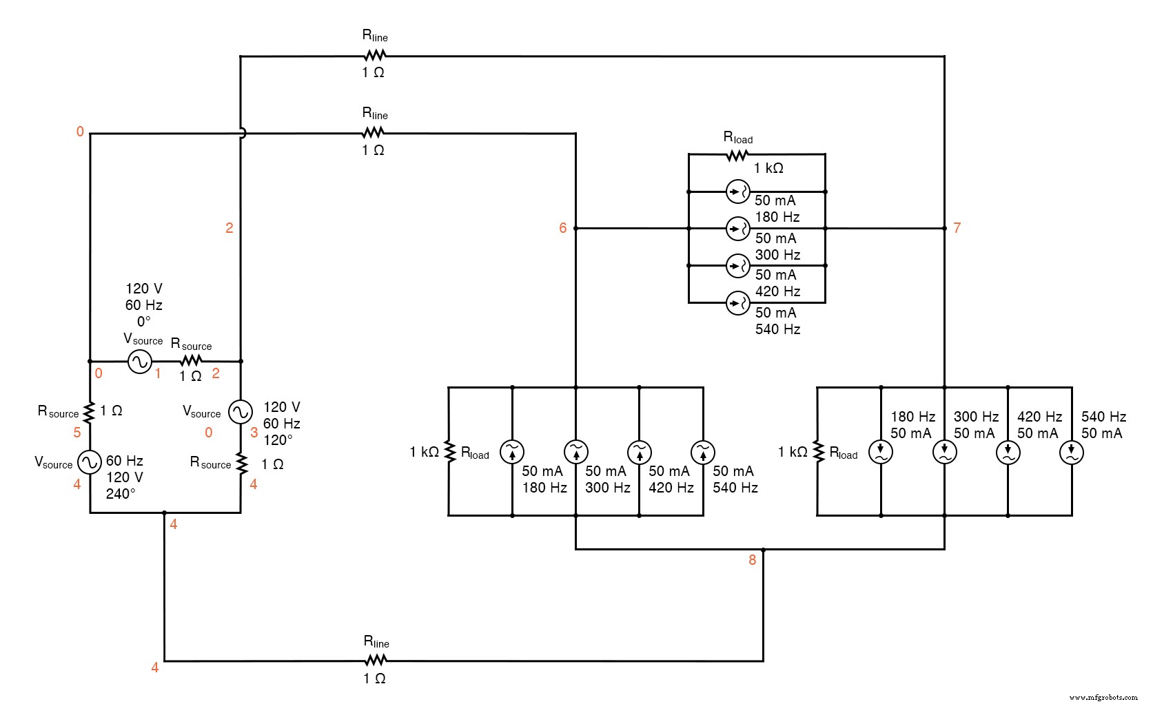
Delta-Delta source/load with harmonics.
Delta-Delta source/load with harmonics * * phase1 voltage source and r (120 v /_ 0 deg) vsource1 1 0 sin(0 120 60 0 0) rsource1 1 2 1 * * phase2 voltage source and r (120 v /_ 120 deg) vsource2 3 2 sin(0 120 60 5.55555m 0) rsource2 3 4 1 * * phase3 voltage source and r (120 v /_ 240 deg) vsource3 5 4 sin(0 120 60 11.1111m 0) rsource3 5 0 1 * * line resistances rline1 0 6 1 rline2 2 7 1 rline3 4 8 1 * * phase 1 of load rload1 7 6 1k i3har1 7 6 sin(0 50m 180 0 0) i5har1 7 6 sin(0 50m 300 0 0) i7har1 7 6 sin(0 50m 420 0 0) i9har1 7 6 sin(0 50m 540 0 0) * * phase 2 of load rload2 8 7 1k i3har2 8 7 sin(0 50m 180 5.55555m 0) i5har2 8 7 sin(0 50m 300 5.55555m 0) i7har2 8 7 sin(0 50m 420 5.55555m 0) i9har2 8 7 sin(0 50m 540 5.55555m 0) * * phase 3 of load rload3 6 8 1k i3har3 6 8 sin(0 50m 180 11.1111m 0) i5har3 6 8 sin(0 50m 300 11.1111m 0) i7har3 6 8 sin(0 50m 420 11.1111m 0) i9har3 6 8 sin(0 50m 540 11.1111m 0) * * analysis stuff .options itl5=0 .tran 0.5m 100m 16m 1u .plot tran v(0,6) v(7,6) v(2,1) i(3har1) .four 60 v(0,6) v(7,6) v(2,1) .Ende
Fourier analysis of line current:
Fourier components of transient response v(0,6) dc component =-6.007E-11 harmonic frequency Fourier normalized phase normalized no (hz) component component (deg) phase (deg) 1 6.000E+01 2.070E-01 1.000000 150.000 0.000 2 1.200E+02 5.480E-11 0.000000 156.666 6.666 3 1.800E+02 6.257E-07 0.000003 89.990 -60.010 4 2.400E+02 4.911E-11 0.000000 8.187 -141.813 5 3.000E+02 8.626E-02 0.416664 -149.999 -300.000 6 3.600E+02 1.089E-10 0.000000 -31.997 -181.997 7 4.200E+02 8.626E-02 0.416669 150.001 0.001 8 4.800E+02 1.578E-10 0.000000 -63.940 -213.940 9 5.400E+02 1.877E-06 0.000009 89.987 -60.013 total harmonic distortion =58.925538 percent
Fourier analysis of load phase voltage:
Fourier components of transient response v(7,6) dc component =-5.680E-10 harmonic frequency Fourier normalized phase normalized no (hz) component component (deg) phase (deg) 1 6.000E+01 1.195E+02 1.000000 0.000 0.000 2 1.200E+02 1.039E-09 0.000000 144.749 144.749 3 1.800E+02 1.251E-06 0.000000 89.974 89.974 4 2.400E+02 4.215E-10 0.000000 36.127 36.127 5 3.000E+02 1.992E-01 0.001667 -180.000 -180.000 6 3.600E+02 2.499E-09 0.000000 -4.760 -4.760 7 4.200E+02 1.992E-01 0.001667 -180.000 -180.000 8 4.800E+02 2.951E-09 0.000000 -151.385 -151.385 9 5.400E+02 3.752E-06 0.000000 89.905 89.905 total harmonic distortion =0.235702 percent
Fourier analysis of source phase current:
Fourier components of transient response v(2,1) dc component =-1.923E-12 harmonic frequency Fourier normalized phase normalized no (hz) component component (deg) phase (deg) 1 6.000E+01 1.194E-01 1.000000 179.940 0.000 2 1.200E+02 2.569E-11 0.000000 133.491 -46.449 3 1.800E+02 3.129E-07 0.000003 89.985 -89.955 4 2.400E+02 2.657E-11 0.000000 23.368 -156.571 5 3.000E+02 4.980E-02 0.416918 -180.000 -359.939 6 3.600E+02 4.595E-11 0.000000 -22.475 -202.415 7 4.200E+02 4.980E-02 0.416921 -180.000 -359.939 8 4.800E+02 7.385E-11 0.000000 -63.759 -243.699 9 5.400E+02 9.385E-07 0.000008 89.991 -89.949 total harmonic distortion =58.961298 percent
As predicted earlier, the load phase voltage is almost a pure sine-wave, with negligible harmonic content, thanks to the direct connection with the source phases in a Δ-Δ system.
But what happened to the triplen harmonics? The 3rd and 9th harmonic frequencies don’t appear in any substantial amount in the line current, nor in the load phase voltage, nor in the source phase current! We know that triplen currents exist because the 3rd and 9th harmonic current sources are intentionally placed in the phases of the load, but where did those currents go?
Analysis of the Effects of Triplen Harmonics in a Delta - Delta Circuit
Remember that the triplen harmonics of 120° phase-shifted fundamental frequencies are in phase with each other.
Note the directions that the arrows of the current sources within the load phases are pointing, and think about what would happen if the 3rd and 9th harmonic sources were DC sources instead.
What we would have is currently circulating within the loop formed by the Δ-connected phases . This is where the triplen harmonic currents have gone:they stay within the Δ of the load, never reaching the line conductors or the windings of the source.
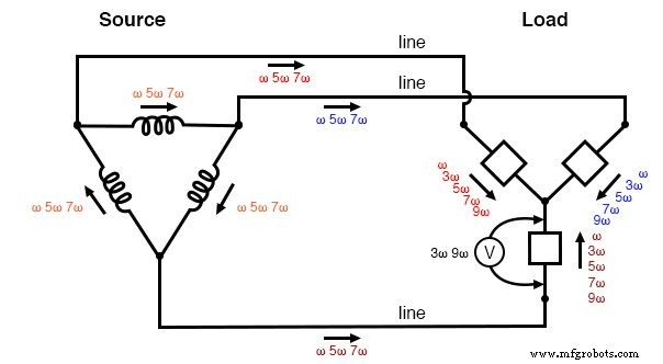
These results may be graphically summarized as such in the figure below.
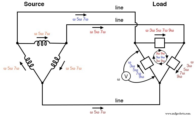
Δ-Δ source/load:Load phases receive undistorted sine wave voltages. Triplen currents are confined to circulate within load phases. Non-triplen currents appear in line conductors and in source phase windings.
This is a major benefit of the Δ-Δ system configuration:triplen harmonic currents remain confined in whatever set of components create them and do not “spread” to other parts of the system.
RÜCKBLICK:
- Nonlinear components are those that draw a non-sinusoidal (non-sine-wave) current waveform when energized by a sinusoidal (sine-wave) voltage. Since any distortion of an originally pure sine-wave constitutes harmonic frequencies, we can say that nonlinear components generate harmonic currents.
- When the sine-wave distortion is symmetrical above and below the average centerline of the waveform, the only harmonics present will be odd-numbered , not even-numbered.
- The 3rd harmonic, and integer multiples of it (6th, 9th, 12th, 15th) are known as triplen harmonics. They are in phase with each other, despite the fact that their respective fundamental waveforms are 120° out of phase with each other.
- In a 4-wire Y-Y system, triplen harmonic currents add within the neutral conductor.
- Triplen harmonic currents in a Δ-connected set of components circulate within the loop formed by the Δ.
VERWANDTE ARBEITSBLÄTTER:
- Mixed-Frequency Signals Worksheet
Industrietechnik
- Einführung in Wechselstromkreise
- Stromquellen
- Zahlensysteme
- Schutzrelais
- Leistungsberechnungen
- Stromsignalsysteme
- Ein kostengünstiges passives Kühlsystem, das keinen Strom benötigt
- Einführung in Oberschwingungen:Teil 2
- Einführung in Harmonische:Teil 1
- Was sind die Haupttypen mechanischer Kraftübertragungssysteme?